
numpy基本使用汇总
简介
-
NumPy代表“Numerical Python”,是一个由多维数组对象和用于处理这些数组的例程(routines)所组成的库。 使用NumPy,可以对数组执行数学和逻辑运算。NumPy不是另一种编程语言,而是Python扩展模块。它对同类数据的数组(array)提供快速有效的操作。 NumPy将Python扩展为用于处理数值数据的高级语言,类似于MATLAB。
-
NumPy主要是用C编写的。这确保了Numpy的数学和数值函数及功能的执行速度。NumPy通过强大的数据结构丰富了编程语言Python,实现了多维数组和矩阵。这些数据结构可确保通过矩阵和数组进行有效的计算。除此之外,该模块还提供了一个庞大的高级数学函数库,可以对这些矩阵和数组进行操作。NumPy是SciPy、Pandas等科学计算或数据处理库的基础。
-
在Python中使用Numpy的优点:
- 面向数组(array)的计算
- 有效实施的多维数组
- 专为科学计算而设计
numpy.ndarray类
- Python已有列表类型,但是如果做运算非常不方便。numpy.ndarray类作为数组对象类型可以实现:
- 数组对象可以去掉元素间运算所需的循环,使一维向量更像单个数据
- 设置专门的数组对象,经过优化,可以提升这类应用的运算速度
- 数组对象采用相同的数据类型,有助于节省运算和存储空间
- ndarray的N维数组类型,它描述了相同类型的元素的集合(collection)。可以使用从零开始的索引来访问集合中的元素。
- 所有ndarray都是同质的(homogenous):每个item占用相同大小的内存块,并且所有块的解释方式都完全相同。数组中各元素的解释方式由一个数据类型对象(称为dtype)指定。除了基本类型(整数,浮点数等)之外,数据类型对象还可以表示数据结构。
内部构成
- ndarray是一个多维数组对象,包括:
- 数据类型对象(dtype):描述这些数据的元数据(数据维度、数据类型等)
- 数组标量(array scalar)类型:实际的数据
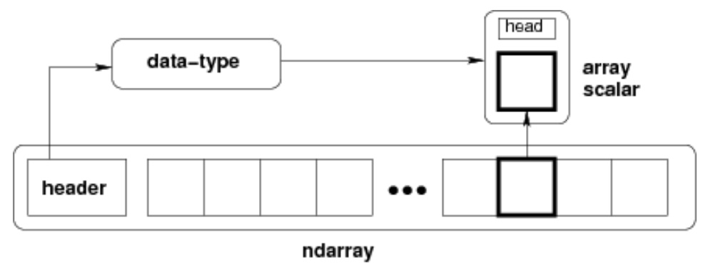
数组标量 (array scalar)
- Python标量非常少,数组标量实现了数据类型的扩充,在大多数情况下它们可以互换使用。
- 使用数组标量的主要优点是它们保留了数组类型(Python可能没有可用的匹配的标量类型,例如int16)。因此,使用数组标量可以确保数组和标量之间的行为相同,而与值是否在数组内部无关。
数据类型对象(dtype)
- 数据类型对象描述了应该如何解释与数组元素相对应的固定大小的内存块中的字节。
- 在dtype的帮助下,我们能够创建“结构化数组”(“Structured Arrays”),也称为“记录数组”(“Record Arrays”)。结构化数组使我们能够为每列提供不同的数据类型。它与excel或csv文档的结构相似。
| 描述 | 说明 |
|---|---|
| 数据类型 | 整数,浮点数,Python对象等 |
| 数据大小 | 以整数为单位的字节数 |
| 数据的字节顺序 | 小端或大端 |
| 如果数据类型是结构化数据类型,则是其他数据类型的集合 | 例如,描述由整数和浮点数组成的一个数组元素 * 该结构的字段(field)的名称是什么,通过它们可以访问它们; * 每个字段的数据类型是什么; * 每个字段占用存储块的哪一部分。 |
| 如果数据类型是子数组(sub-array),则其形状和数据类型是什么 |
大端序和小端序
-
大端模式 (big-endian):是指数据的高字节保存在内存的低地址中,而数据的低字节保存在内存的高地址中,这样的存储模式有点儿类似于把数据当作字符串顺序处理:地址由小向大增加,而数据从高位往低位放;这和我们的阅读习惯一致。
-
小端模式 (little-endian):是指数据的高字节保存在内存的高地址中,而数据的低字节保存在内存的低地址中,这种存储模式将地址的高低和数据位权有效地结合起来,高地址部分权值高,低地址部分权值低,和我们的逻辑方法一致。
-
例如一个16bit的short型x,在内存中的地址为0x0010,x的值为0x1122,那么0x11为高字节,0x22为低字节。
- 对于大端模式,就将0x11放在低地址中,即0x0010中,0x22放在高地址中,即0x0011中。
- 小端模式,刚好相反。
-
我们常用的X86结构是小端模式,而KEIL C51则为大端模式。很多的ARM,DSP都为小端模式。
dtype类型
| dtype类型 | 说明 |
|---|---|
| dt = np.dtype(‘b’) | byte, native byte order |
| dt = np.dtype(’>H’) | big-endian unsigned short |
| dt = np.dtype(’<f’) | little-endian single-precision float |
| dt = np.dtype(‘d’) | double-precision floating-point number |
| dt = np.dtype(‘i4’) | 32-bit signed integer |
| dt = np.dtype(‘f8’) | 64-bit floating-point number |
| dt = np.dtype(‘c16’) | 128-bit complex floating-point number |
| dt = np.dtype(‘a25’) | 25-length zero-terminated bytes |
| dt = np.dtype(‘U25’) | 25-character string |
| dt = np.dtype(“i4, (2,3)f8, f4”) | * field named f0 containing a 32-bit integer * field named f1 containing a 2 x 3 sub-array of 64-bit floating-point numbers * field named f2 containing a 32-bit floating-point number |
dtype属性
- dt = np.dtype(’>i4’)
| dtype属性 | 说明 |
|---|---|
| dt.byteorder | ‘>’:大端序小端序判断 |
| dt.itemsize | 4:每项数据的字节大小 |
| dt.name | int32:类型名称 |
| dt.type is np.int32 | True:对应的np类型 |
dtype使用
import numpy as np |
ndarray对象
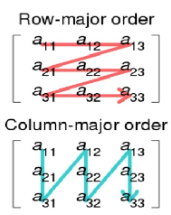
- ndarray对象由计算机内存中连续一维segment组成,并与将每个元素映射到内存块中某个位置的索引方案结合在一起。内存块按行优先顺序(C style)或列优先顺序(FORTRAN或MatLab style)保存元素。
- ndarray的数组是“ N维数组”的简写。N维数组只是具有任意数量维度的数组。用于表示矩阵和向量。
| 维度 | 表述 |
|---|---|
| 一维数组 | 向量,分为行向量和列向量 |
| 两维数组 | 矩阵 |
| 三维或更高维数组 | 通常使用张量(tensor)这一术语 |
数组属性
- 数组通常是具有相同类型和大小的元素的固定大小的容器。数组属性反映了数组本身固有的信息。
| 属性 | 说明 |
|---|---|
| ndarray.ndim | 秩,即轴的数量或维度的数量 |
| ndarray.shape | 数组的维度,对于矩阵,n 行 m 列 |
| ndarray.size | 数组元素的总个数,相当于 .shape 中 n* m 的值 |
| ndarray.dtype | ndarray 对象的元素类型 |
| ndarray.itemsize | ndarray 对象中每个元素的大小,以字节为单位 |
| ndarray.flags | ndarray 对象的内存信息 |
| ndarray.real | ndarray元素的实部 |
| ndarray.imag | ndarray 元素的虚部 |
| ndarray.data | 包含实际数组元素的缓冲区。由于一般通过数组的索引获取元素,通常不需要使用这个属性。 |
shape
- 数组中的维数和元素数由其形状(shape)定义。
axes
- 在NumPy中,不同的维度称为轴(axes)。
[[0., 0., 0.], [1., 1., 1.]]
- 该数组有2个轴。第一轴的长度为2,第二轴的长度为3。
- 在二维NumPy数组中,轴是沿行和列的方向。 axis=0,表示沿着第 0 轴(行的方向)进行操作;axis=1,表示沿着第1轴进行操作。
rank
- NumPy 数组的维数称为秩(rank),秩就是轴的数量,即数组的维度,一维数组的秩为 1,二维数组的秩为 2
dimensions
- 在 NumPy中,每一个线性的数组称为是一个轴(axis),也就是维度(dimensions)。比如说,二维数组相当于是两个一维数组,其中第一个一维数组中每个元素又是一个一维数组。所以一维数组就是 NumPy 中的轴(axis),第一个轴相当于是底层数组,第二个轴是底层数组里的数组。而轴的数量——秩,就是数组的维数。
itemsize
- ndarray.itemsize 以字节的形式返回数组中每一个元素的大小。
- 例如,一个元素类型为 float64 的数组 itemsize 属性值为 8(float64 占用 64 个 bits,每个字节长度为 8,所以 64/8,占用 8 个字节);
- 又如,一个元素类型为 complex32 的数组 itemsize 属性值为 4(32/8)。
flags
- ndarray.flags 返回 ndarray 对象的内存信息,包含以下属性:
| 属性 | 描述 |
|---|---|
| C_CONTIGUOUS © | 数据是在一个单一的C风格的连续段中 |
| F_CONTIGUOUS (F) | 数据是在一个单一的Fortran风格的连续段中 |
| OWNDATA (O) | 数组拥有它所使用的内存或从另一个对象中借用它 |
| WRITEABLE (W) | 数据区域可以被写入,将该值设置为 False,则数据为只读 |
| ALIGNED (A) | 数据和所有元素都适当地对齐到硬件上 |
| UPDATEIFCOPY (U) | 这个数组是其它数组的一个副本,当这个数组被释放时,原数组的内容将被更新 |
numpy.mat类
- Numpy中有“真正的”矩阵(Matrix)。 它们是二维数组的子集。 我们可以通过应用mat函数将一个二维数组转换为一个矩阵。
- 与Numpy的二维数组主要区别在于将两个二维数组或两个矩阵相乘时,两个矩阵相乘得到真正的乘法,但二维数组相乘只是逐元素相乘
A = np.array([ [1, 2, 3], [2, 2, 2], [3, 3, 3] ]) |
数组
创建
np.array()
-
自定义数组,简单数组所需要做的就是将列表传递给它,使用dtype关键字明确指定要使用的数据类型。
-
a = np.array([1, 2, 3], dtype=np.int64) -
创建标量42。将ndim方法应用于标量,得到数组的维度为0
-
x = np.array(42)
np.ones()
-
全1向量
-
x = np.ones(2) # [1.,1.] -
全1数组
-
x = np.ones((1,1))
np.zeros()
-
全0向量
-
x = np.zeros(2) # [1.,1.] -
全0数组
-
x = np.zeros((1,1))
np.ones_like() np.zeros_like()
- 产生的数组与另一个现有数组具有相同的形状
x = np.array([2,5,18,14,4])E = np.ones_like(x)Z = np.zeros_like(x)
np.empty()
- 创建并返回对给定形状和类型的新数组的引用,而不初始化元素,注意通常它们是任意值。
np.empty((2, 4))
np.arange()
arange([start,] stop[, step], [, dtype=None])np.arange(1, 10)- 在给定间隔内返回均匀间隔的值
- 返回数组是半开区间[start,stop)内生成的,如果未给出start参数,则将其设置为0。
- 间隔的结束由参数stop确定。通常,间隔不包括此值,除非在某些情况下step不是整数,浮点舍入会影响输出ndarray的长度。
- 使用可选参数step设置输出数组的两个相邻值之间的间距。 step的默认值是1。如果给出参数step,start参数不能是可选的,即它也必须给出。
- 可以使用参数dtype指定输出数组的类型。如果未给出,则将从其他输入参数自动推断类型。
np.linspace()
-
linspace(start, stop, num=50, endpoint=True, retstep=False) -
linspace返回一个ndarray,由闭区间[start,stop]或半开区间[start,stop]中的num个等间隔样本组成。返回闭或半开间隔,则取决于endpoint是True还是False。
-
参数start定义将要创建的序列的起始值。
-
stop将是序列的结束值,除非endpoint设置为False。 在后一种情况下,得到的序列将由除num+1个样本外的均匀间隔的样本组成。 这意味着排除stop。
-
请注意,当endpoint为False时,步长会发生变化。
-
可以使用num设置要生成的样本数,默认为50。如果可选参数endpoint设置为True(默认值),stop将是序列的最后一个样本。 否则,它不包括在内。
-
如果设置了可选参数retstep,则该函数还将返回相邻值之间的间距值。 因此,该函数将返回一个元组(‘samples’, ‘step’):
-
samples, spacing = np.linspace(1, 10, 20, endpoint=True, retstep=True)
np.identity()
- 单位方阵
identity(n, dtype=None),输出是nxn数组,其主对角线设置为1,所有其他元素为0- n:一个整数,用于定义输出的行数和列数,即nxn
- dtype:一个可选参数,用于定义输出的数据类型。 默认为float
np.eye()
- 创建仅由1组成的对角线数组
eye(N, M=None, k=0, dtype=float),返回一个形状的(N,M)的ndarray。 除了第k个对角线为1之外,该数组的所有元素都等于零。- N定义输出数组行的整数。
- M一个可选的整数,用于设置输出中的列数。 如果为None,则默认为“N”。
- k定义对角线的位置。 默认值为0。0表示主对角线。 正值表示上对角线,负值表示下对角线。
- dtype返回数组的可选数据类型。
复制
np.copy()
-
返回给定对象obj的数组拷贝
copy(obj, order='K')- obj:array_like输入数据。
- order:可能的值是{‘C’,‘F’,‘A’,‘K’}。 此参数控制拷贝的内存布局。
- 'C’表示C顺序,
- 'F’表示Fortran顺序:Fortran数组是列优先的。
- 如果对象obj是Fortran连续的’A’表示’F’,否则表示’C’。 'K’表示尽可能匹配obj的布局。
-
x = np.array([[42],[44]], order='F') -
y = np.copy(x)
ndarray.copy()
- 它与np.copy()类似,但顺序参数的默认值不同
a.copy(order='C')
浅拷贝
a = np.arange(12)b = a- a b只是变量名不同,指向内容相同
视图
c = a.view()- 创建一个新的数组对象,共享相同的数据,改变shape不会相互影响,而修改数据则会直接反馈到原始对象
- c.flags.owndata是false
访问
索引
- 一维数组
data = np.array([1, 2, 3]) |
- 多维数组
A = np.array([ [3.4, 8.7, 9.9], |
切片
- python在列表和元组上的切片会创建新对象,但对ndarray数组执行切片操作会在原始数组上创建一个视图(view)。 如果我们修改一个视图,原始数组也将被修改。
A = np.array([0, 1, 2, 3, 4, 5, 6, 7, 8, 9]) |
- 多维数组
- 如果选择元组中的对象数目小于维N,则对于任何后续维度的假定是’:’
a = np.arange(40).reshape(5, 8) |
高级索引
布尔数组
- 测试数组A的每个元素, 看其是否等于4。这些测试的结果是结果数组的布尔元素。
A = np.array([4, 7, 3, 4, 2, 8]) |
- 这对图像进行阈值非常方便
A = np.array([ |
花式索引
- 用布尔数组或整数数组(掩码,mask)对数组进行索引,则称为花式索引。 结果将是一个拷贝(副本)而不是一个视图。
C = np.array([123,188,190,99,77,88,100]) |
整数数组索引
C[[0, 2, 3, 1, 4, 1]] |
- 多维索引
a = np.arange(40).reshape(5, 8) |
np.nonzero() ndarray.nonzero()
- 以数组的元组形式返回非零的a元素的索引
a[a.nonzero()] |
np.where()
np.where(condition, x, y)满足条件(condition),输出x,不满足输出y。
a = np.arange(10) |
-
上面这个例子的条件为[[True,False], [True,False]],分别对应最后输出结果的四个值。第一个值从[1,9]中选,因为条件为True,所以是选1。第二个值从[2,8]中选,因为条件为False
-
np.where(condition)只有条件 (condition),没有x和y,则输出满足条件 (即非0) 元素的坐标 (等价于numpy.nonzero)
运算
加减乘除
标量
- 标量运算将作用到每个元素中
v = np.array([2,3, 7.9, 3.3, 6.9, 0.11, 10.3, 12.9]) |
数组间
- 如果有两个相同大小的矩阵,两个数组间操作,则将按逐元素方式组合,所以A * B不应该被误认为是矩阵乘法。 这些元素只是逐元素相乘。
data = np.array([1, 2]) |
点积
np.dot()
dot(a, b, out=None)- 要求a的最后一个维度的形状与b的倒数第二个维度的形状的相同,即要求a.shape[-1] == b.shape[-2],否则会引发ValueError
比较
- 比较两个数组,比较是按元素进行的,返回一个布尔数组
np.array_equal()
- 比较数组是否完整的相等,具有相同的形状和相同的元素。我们使用array_equal来实现此目的。
np.array_equal(A, B) |
逻辑
np.logical_or()
np.logical_and()
操作
展平数组
ndarray.flatten()
ndarray.flatten([order='C'])- order可以具有值“ C”、“ F”、“A”和“K”。 默认顺序为“C”。
- “C”表示C-style按row-major ordering(行主顺序)展平,即最右边的索引更改最快,换句话说:按行主顺序,行索引变化最慢,列索引变化最快,因此 a[0,0]接着的是a[0,1]。
- “F”代表Fortran-style的列主顺序。
- “A”表示如果数组在内存中是连续的,则按列优先顺序进行展平;否则,按行优先进行展平。
- “K”表示按数组元素在内存中出现的顺序展平。
a = np.arange(24).reshape((3,4,2)) |
ndarray.ravel()
ravel(a, order='C')仅返回原始数组的reference/view,flatten返回原始数组的副本- 等价于
reshape(-1, order=order) - ravel是库级别的函数,因此可以在任何可以成功解析的对象上调用。flatten是ndarray对象的方法,所以ravel将在ndarray列表上工作,而flatten不适用于该类型的对象。
- ravel比flatten()更快,因为它不占用任何内存。
reshape
reshape(a, newshape, order='C')在不更改数据的情况下为一个数组提供了新的形状,即返回具有新形状的一个视图。
更改维度
np.newaxis()
- 用于创建长度为1的轴。 newaxis是None的别名,可以用None代替它,结果相同
a = np.array([1, 2, 3, 4, 5]) # (5,) |
np.expand_dims()
- 扩展数组的形状,可以插入一个新的轴,该轴出现在扩展数组形状的轴位置上。
a = np.array([2, 4]) # (2,) |
np.squeeze()
- 从一个数组的形状中去除一维条目。
x = np.array([[[0], [1], [2]]]) # (1, 3, 1) |
广播
- 前面数组运算包含了标量和大小相同数组间的加减乘除,对于不同的形状的两个数组,Numpy提供了一种称为广播(Broadcasting)的强大机制进行算数运算。
- 这意味着我们有一个较小的数组和一个较大的数组,我们多次转换或应用较小的数组,以对较大的数组执行某些操作。 换句话说:在某些条件下,较小的数组被“广播”成与较大数组具有相同的形状。借助广播,我们可以避免Python程序中的循环。 循环在Numpy实现中隐式发生。还可以避免了创建不必要的数据副本。
data = np.array([1.0, 2.0]) |
- 对不同大小的矩阵执行这些算术运算,但前提是一个矩阵只有一列或一行。在这种情况下,NumPy将使用其广播规则进行操作。
data = np.array([[1, 2], [3, 4], [5, 6]]) |
- 举例:距离矩阵 (Distance Matrix)
dist2barcelona = [0, 1498, 1063, 1968,1498, 1758, 1469, 1472, 2230, 2391, 1138, 505, 725, 3007, 1055, 833, 1354, 857, 2813, 2277, 1347, 1862] |
tile
- 重复模式 (Repeating Patterns),重复现有矩阵多次来创建具有不同形状甚至维度的新矩阵。
tile(A, reps)- 通过把A重复reps次数来构造一个数组。reps通常是一个元组(或列表),用于定义沿相应轴/方向的重复次数。
x = np.array([ [1, 2], [3, 4]]) |
- 如果我们坚持以元组或列表形式写reps,或者将reps = 5表示为reps = (5,)的缩写,则以下内容是正确的:
- 如果reps的长度为n,则结果数组的维数将为n和A.ndim的最大值。
- 如果A.ndim < n,则通过添加新轴将A提升为n维。 因此,将形状(5,)数组提升为(1, 5) 以进行2D复制,或将形状(1, 1, 5)提升为3D复制。
- 如果A.ndim > d,则将reps前置1提升为’A’.ndim。
- 因此,对于形状为(2, 3, 4, 5)的数组“ A”,一个(2, 2)的“ reps”被视为(1, 1, 2, 2)。
转置
transpose
ndarray.T
rollaxis
numpy.rollaxis(arr, axis, start)- 此函数使指定的轴滚动,直到它位于指定的位置。 该函数具有三个参数。
- arr:输入数组
- axis:滚动的轴。 其他轴的位置相对彼此不变
- start:默认为0来完成整个滚动。 滚动直到到达指定位置
a = np.arange(8).reshape(2,2,2) # [[[0 1][2 3]][[4 5][6 7]]] |
- 程序运行np.rollaxis(a, 2)时, 将轴2滚动到了轴0前面,数组下标排序由0,1,2变成了1,2,0。其他轴相对2轴位置不变(start默认0)。
0(000)->0(000) 1(001)->2(010) |
- 程序运行np.rollaxis(a, 2, 1)时,将轴2滚动到了轴1前面,数组下标排序由0,1,2变成了0,2,1。
swapaxes
numpy.swapaxes(arr, axis1, axis2)- 交换,将axis1和axis2进行互换
a = np.array([[2,3,4]]) |
翻转
np.flip(m, axis=None)
- numpy.flip(m, axis=None)
- 沿给定轴颠倒数组中元素的顺序
- 数组的形状被保留,但是元素被重新排序。
| 方法 | 说明 |
|---|---|
| flip(m, 0) | 上下翻转 is equivalent to flipud(m). |
| flip(m, 1) | 左右翻转 is equivalent to fliplr(m). |
| flip(m, n) | corresponds to m[…,::-1,…] with ::-1 at position n. |
| flip(m) | corresponds to m[::-1,::-1,…,::-1] with ::-1 at all positions. |
| flip(m, (0, 1)) | corresponds to m[::-1,::-1,…] with ::-1 at position 0 and position 1. |
A = np.arange(8).reshape((2,2,2)) # array([[[0, 1],[2, 3]],[[4, 5],[6, 7]]]) |
拼接
np.concatenate
- 沿指定轴拼接相同形状的两个或多个数组
- 默认axis=0拼接
a = np.array([[1,2],[3,4]]) |
堆叠
np.stack
- 沿新轴堆叠若干个数组
a = np.array([[1,2],[3,4]]) # [[1,2],[3,4]] |
np.hstack
- 通过水平堆叠来生成数组
c = np.hstack((a,b)) # [[1 2 5 6][3 4 7 8]] (2, 4) |
np.vstack
- 通过垂直堆叠来生成数组
c = np.vstack((a,b)) # [[1 2][3 4][5 6][7 8]] (4, 2) |
np.c_[x,y]
- 将切片对象沿第二个轴(列)拼接,相当于增加了维度,再np.hstack
np.c_[np.array([1,2,3]),np.array([4,5,6])] # [[1 4][2 5][3 6] |
np.r_[x,y]
- 将切片对象沿第一个轴(行)拼接
np.r_[np.array([1,2,3]),0,0,np.array([4,5,6])] # [[1 2 3 0 0 4 5 6]] |
分割
np.split
- 沿特定的轴将数组分割为子数组
numpy.split(ary, indices_or_sections, axis)- ary:被分割的数组
- indices_or_sections:如果是一个整数,就用该数平均切分;如果是一个数组,为沿轴切分的位置
- axis:沿着哪个维度进行切分。默认为0,横向切分。为1时,纵向切分。
a = np.arange(9) |
np.hsplit
- 用于水平分割数组,通过指定要返回的相同形状的数组数量来拆分原数组。
np.vsplit
修改大小
np.resize
- 返回指定大小的新数组。如果新数组大小大于原始大小,则包含原始数组中的元素的副本。
numpy.resize(arr, shape)- arr:要修改大小的数组
- shape:返回数组的新形状
a = np.array([[1,2,3],[4,5,6]]) |
添加
append
- 在数组的末尾添加值。 追加操作会分配整个数组,并把原来的数组复制到新数组中。 此外,输入数组的维度必须匹配否则将生成ValueError。
numpy.append(arr, values, axis=None)- arr:输入数组
- value:要向arr添加的值,需要和arr形状相同(除了要添加的轴)
- axis:默认为 None。当axis无定义时,是横向添加,返回总是为一维数组。当axis有定义的时候,分别为0和1的时候。当axis为0时,数组是加在下边(列数要相同)。当axis为1时,数组是加在右边(行数要相同)。
a = np.array([[1,2,3],[4,5,6]]) |
insert
- 在给定索引之前,沿给定轴在输入数组中插入值。
numpy.insert(arr, obj, values, axis)- arr:输入数组
- obj:在其之前插入值的索引
- values:要插入的值
- axis:沿着它插入的轴,如果未提供,则输入数组会被展开
a = np.array([[1,2],[3,4],[5,6]]) |
删除
delete
- 返回从输入数组中删除指定子数组的新数组。 与 insert() 函数的情况一样,如果未提供轴参数,则输入数组将展开。
Numpy.delete(arr, obj, axis)- arr:输入数组
- obj:可以被切片,整数或者整数数组,表明要从输入数组删除的子数组
- axis:沿着它删除给定子数组的轴,如果未提供,则输入数组会被展开
a = np.arange(12).reshape(3,4) |
unique
- 用于去除数组中的重复元素。
numpy.unique(arr, return_index, return_inverse, return_counts)- arr:输入数组,如果不是一维数组则会展开
- return_index:如果为true,返回新列表元素在旧列表中的位置(下标),并以列表形式储存
- return_inverse:如果为true,返回旧列表元素在新列表中的位置(下标),并以列表形式储存
- return_counts:如果为true,返回去重数组中的元素在原数组中的出现次数
a = np.array([5,2,6,2,7,5,6,8,2,9]) |
np.nditer()
单数组迭代
- 迭代数组
- a和a.T的元素以相同的顺序遍历,即按照它们存储在内存中的顺序;而a.T.copy(order=’C’)的元素以不同的顺序访问,因为它们被放入了不同的内存布局。
a = np.arange(6).reshape(2,3) |
控制迭代顺序
for x in np.nditer(a, order='F'): # 列序优先 |
修改数组值
- 默认情况下,nditer将输入操作数视为只读对象。 为了能够修改数组元素,必须使用每个操作数标志readwrite或writeonly指定读写模式或只写模式。
- 然后,nditer将产生可以修改的可写缓冲区数组。 但是,由于nditer必须在迭代完成后将此缓冲区数据复制回原始数组,因此必须使用两种方法之一通知结束迭代的时间。
- 使用with语句将nditer用作上下文管理器,退出上下文时将写回临时数据。
- 迭代完成后,调用迭代器的close方法,这将触发回写。
- 一旦调用close或退出其上下文,nditer将无法再进行迭代。
with np.nditer(a, op_flags=['readwrite']) as it: |
广播数组迭代
a = np.arange(3) |
maskedarray
- 掩码数组(Masked arrays)是可能缺少条目或无效条目的数组。
创建掩码数组
x = np.array([1, 2, 3, -99, 5]) |
修改掩码
- 可以通过赋值来修改掩码:
mx[1] = np.ma.masked |
- 可以使用一个给定的值填充被掩码的条目,以获取通常的数组:
x2 = mx.filled(-1) |
清除掩码
mx.mask = np.ma.nomask |
结构化数组
- ndarray是同质的数据对象,即数组的所有元素必须是相同的数据类型。 另一方面,数据类型dytpe允许为每列定义单独的数据类型。
- 结构化数组是这样的ndarray,其数据类型是由较简单数据类型组合成的命名字段的序列(a sequence of named fields)。
x = np.array([('Rex', 9, 81.0), ('Fido', 3, 27.0)],dtype=[('name', 'U10'), ('age', 'i4'), ('weight', 'f4')]) |
创建
- 可以使用函数numpy.dtype创建结构化数据类型。有4种可选的形式,其灵活性和简洁性各不相同。
# 方法一:A list of tuples, one tuple per field |
通用函数(ufunc)
- 通用函数(简称ufunc)是一种以逐元素的方式在ndarray上操作的函数,支持数组广播、类型转换和其他几个标准功能。 也就是说,ufunc是函数的“向量化”包装器(“vectorized” wrapper),该函数采用固定数量的特定输入并产生固定数量的特定输出。
| 方法 | 说明 |
|---|---|
| ufunc.reduce(a[, axis, dtype, out, …]) | Reduces a’s dimension by one, by applying ufunc along one axis. |
| ufunc.accumulate(array[, axis, dtype, out]) | Accumulate the result of applying the operator to all elements. |
| ufunc.reduceat(a, indices[, axis, dtype, out]) | Performs a (local) reduce with specified slices over a single axis. |
| ufunc.outer(A, B, **kwargs) | Apply the ufunc op to all pairs (a, b) with a in A and b in B. |
| ufunc.at(a, indices[, b]) | Performs unbuffered in place operation on operand ‘a’ for elements specified by ‘indices’. |
ufunc.reduce(a[, axis, dtype, out, …])
- Reduces a’s dimension by one, by applying ufunc along one axis.
a = np.array([1,2,3,4]) |
ufunc.accumulate(array[, axis, dtype, out])
- Accumulate the result of applying the operator to all elements.
a = np.array([1,2,3,4]) |
ufunc.reduceat(a, indices[, axis, dtype, out])
- Performs a (local) reduce with specified slices over a single axis.
a = np.array( |
ufunc.outer(A, B, **kwargs)
- Apply the ufunc op to all pairs (a, b) with a in A and b in B.
ufunc.at(a, indices[, b])
- Performs unbuffered in place operation on operand ‘a’ for elements specified by ‘indices’.
算术操作 (Math operations)
| 操作 | 描述 |
|---|---|
| add(x1, x2, /[, out, where, casting, order, …]) | Add arguments element-wise. |
| subtract(x1, x2, /[, out, where, casting, …]) | Subtract arguments, element-wise. |
| multiply(x1, x2, /[, out, where, casting, …]) | Multiply arguments element-wise. |
| divide(x1, x2, /[, out, where, casting, …]) | Returns a true division of the inputs, element-wise. |
三角函数 (Trigonometric functions)
- 当用角度时,所有三角函数都使用弧度。 度与弧度的比率为180/pi。
| 操作 | 描述 |
|---|---|
| sin(x, /[, out, where, casting, order, …]) | Trigonometric sine, element-wise. |
| cos(x, /[, out, where, casting, order, …]) | Cosine element-wise. |
| tan(x, /[, out, where, casting, order, …]) | Compute tangent element-wise. |
比特操作函数 (Bit-twiddling functions)
- These function all require integer arguments and they manipulate the bit-pattern of those arguments.
| 操作 | 描述 |
|---|---|
| bitwise_and(x1, x2, /[, out, where, …]) | Compute the bit-wise AND of two arrays element-wise. |
| bitwise_or(x1, x2, /[, out, where, casting, …]) | Compute the bit-wise OR of two arrays element-wise. |
| bitwise_xor(x1, x2, /[, out, where, …]) | Compute the bit-wise XOR of two arrays element-wise. |
比较函数 (Comparison functions)
| 操作 | 描述 |
|---|---|
| greater(x1, x2, /[, out, where, casting, …]) | Return the truth value of (x1 > x2) element-wise. |
| greater_equal(x1, x2, /[, out, where, …]) | Return the truth value of (x1 >= x2) element-wise. |
| less(x1, x2, /[, out, where, casting, …]) | Return the truth value of (x1 < x2) element-wise. |
| less_equal(x1, x2, /[, out, where, casting, …]) | Return the truth value of (x1 =< x2) element-wise. |
| not_equal(x1, x2, /[, out, where, casting, …]) | Return (x1 != x2) element-wise. |
| equal(x1, x2, /[, out, where, casting, …]) | Return (x1 == x2) element-wise. |
浮点函数 (Floating functions)
| 操作 | 描述 |
|---|---|
| isfinite(x, /[, out, where, casting, order, …]) | Test element-wise for finiteness (not infinity or not Not a Number). |
| isinf(x, /[, out, where, casting, order, …]) | Test element-wise for positive or negative infinity. |
| isnan(x, /[, out, where, casting, order, …]) | Test element-wise for NaN and return result as a boolean array. |
| isnat(x, /[, out, where, casting, order, …]) | Test element-wise for NaT (not a time) and return result as a boolean array. |
| fabs(x, /[, out, where, casting, order, …]) | Compute the absolute values element-wise. |
| nan_to_num(x, [num]) | 将nan替换为num,默认nan替换为0,inf替换为极大值1e308 |
聚合函数
| 操作 | 描述 |
|---|---|
| sum(a[, axis]) | 求和,Sum of array elements over a given axis. |
| prod(a[, axis]) | 求积Return the product of array elements over a given axis. |
| diff(a[, n, axis]) | Calculate the n-th discrete difference along given axis. |
| cumsum(a[, axis, dtype, out]) | Return the cumulative sum of the elements along a given axis. |
np.sum([0.5, 1.5]) # 2 |
指数操作
| 操作 | 描述 |
|---|---|
| exp(x, /[, out, where, casting, order, …]) | Calculate the exponential of all elements in the input array. |
| log(x, /[, out, where, casting, order, …]) | Natural logarithm, element-wise |
| log10(x, /[, out, where, casting, order, …]) | Return the base 10 logarithm of the input array, element-wise. |
| log2(x, /[, out, where, casting, order, …]) | Base-2 logarithm of x |
统计函数
Averages and variances
| 操作 | 说明 |
|---|---|
| median(a[, axis, out, overwrite_input, keepdims]) | Compute the median (中位数) along the specified axis.如果数据的个数是奇数,则中间那个数据就是这群数据的中位数;如果数据的个数是偶数,则中间那2个数据的算术平均值就是这群数据的中位数。 |
| average(a[, axis, weights, returned]) | Compute the weighted average (加权平均值)along the specified axis. np.average(np.array([1,2,3,4]), weights=np.array([1,2,3,4])) |
| mean(a[, axis, dtype, out, keepdims]) | Compute the arithmetic mean (算术平均值) along the specified axis. |
| std(a[, axis, dtype, out, ddof, keepdims]) | Compute the standard deviation (标准差)along the specified axis. |
| var(a[, axis, dtype, out, ddof, keepdims]) | Compute the variance (方差)along the specified axis. |
| nanmedian(a[, axis, out, overwrite_input, …]) | Compute the median along the specified axis, while ignoring NaNs. |
| nanmean(a[, axis, dtype, out, keepdims]) | Compute the arithmetic mean along the specified axis, ignoring NaNs. |
| nanstd(a[, axis, dtype, out, ddof, keepdims]) | Compute the standard deviation along the specified axis, while ignoring NaNs. |
| nanvar(a[, axis, dtype, out, ddof, keepdims]) | Compute the variance along the specified axis, while ignoring NaNs. |
Order statistics
| 操作 | 说明 |
|---|---|
| amin(a[, axis, out, keepdims, initial, where]) | Return the minimum of an array or minimum along an axis. |
| amax(a[, axis, out, keepdims, initial, where]) | Return the maximum of an array or maximum along an axis. |
| nanmin(a[, axis, out, keepdims]) | Return minimum of an array or minimum along an axis, ignoring any NaNs. |
| nanmax(a[, axis, out, keepdims]) | Return the maximum of an array or maximum along an axis, ignoring any NaNs. |
| ptp(a[, axis, out, keepdims]) | Range of values (maximum - minimum) along an axis.返回最大值-最小值,用于归一化 |
| percentile(a, q[, axis, out, …]) | Compute the q-th percentile of the data along the specified axis.一组n个观测值按数值大小排列。处于p%位置的值称第p百分位数。 如果p = 50,此函数与中位数相同;如果p = 0,则与最小值相同;如果p = 100,则与最大值相同。 |
| nanpercentile(a, q[, axis, out, …]) | Compute the qth percentile of the data along the specified axis, while ignoring nan values. |
| quantile(a, q[, axis, out, overwrite_input, …]) | Compute the q-th quantile of the data along the specified axis. |
| nanquantile(a, q[, axis, out, …]) | Compute the qth quantile of the data along the specified axis, while ignoring nan values. |
Correlating
| 操作 | 说明 |
|---|---|
| corrcoef(x[, y, rowvar, bias, ddof]) | Return Pearson product-moment correlation coefficients.相关系数,得到归一化的相关矩阵 |
| correlate(a, v[, mode]) | Cross-correlation of two 1-dimensional sequences. 互相关,计算方法固定a,移动v,计算他们重合部分的累加积,取最大值。mode:same完全和错一位 valid完全重叠 full所有情况 |
| cov(m[, y, rowvar, bias, ddof, fweights, …]) | Estimate a covariance matrix, given data and weights. |
Histograms
| 操作 | 说明 |
|---|---|
| histogram(a[, bins=np.arange(10), range, normed, weights, density=False, …]) | Compute the histogram of a set of data. density:false返回统计数量,true返回归一化的值 |
| histogram2d(x, y[, bins, range, normed, …]) | Compute the bi-dimensional histogram of two data samples. |
| histogramdd(sample[, bins, range, normed, …]) | Compute the multidimensional histogram of some data. |
| bincount(x[, weights, minlength]) | Count number of occurrences of each value in array of non-negative ints. |
| histogram_bin_edges(a[, bins, range, weights]) | Function to calculate only the edges of the bins used by the histogram function. |
| digitize(x, bins[, right=False]) | Return the indices of the bins to which each value in input array belongs.将数值,根据区间bin,right是否包含最右,生成对应区间索引 |
排序函数
| 操作 | 说明 |
|---|---|
| sort(a[, axis, kind, order]) | Return a sorted copy of an array.axis默认是按照最后一个轴排序,order是根据某个字段排序 |
| lexsort(keys[, axis]) | Perform an indirect stable sort using a sequence of keys. |
| argsort(a[, axis, kind, order]) | Returns the indices that would sort an array. 返回排序后的索引数组 |
| ndarray.sort([axis, kind, order]) | Sort an array in-place. |
| msort(a) | Return a copy of an array sorted along the first axis. |
| sort_complex(a) | Sort a complex array using the real part first, then the imaginary part. |
| partition(a, kth[, axis, kind, order]) | Return a partitioned copy of an array. |
| argpartition(a, kth[, axis, kind, order]) | Perform an indirect partition along the given axis using the algorithm specified by the kind keyword. |
条件查找
| 操作 | 说明 |
|---|---|
| argmax(a[, axis, out]) | Returns the indices of the maximum values along an axis. |
| nanargmax(a[, axis]) | Return the indices of the maximum values in the specified axis ignoring NaNs. |
| argmin(a[, axis, out]) | Returns the indices of the minimum values along an axis. |
| nanargmin(a[, axis]) | Return the indices of the minimum values in the specified axis ignoring NaNs. |
| argwhere(a) | Find the indices of array elements that are non-zero, grouped by element. |
| nonzero(a) | Return the indices of the elements that are non-zero. |
| flatnonzero(a) | Return indices that are non-zero in the flattened version of a. |
| where(condition, [x, y]) | Return elements chosen from x or y depending on condition. np.where(a < 5, a, 10*a) |
| searchsorted(a, v[, side, sorter]) | Find indices where elements should be inserted to maintain order.a是排好序的数组,在a中检索v所处的位置,默认从左开始检索,side=left左开右闭,side=right左闭右开。可以用于按照比例的随机选择:a[np.searchsorted(np.r_[np.linspace(0,0.5,num=50),np.linspace(0.5,0.75,num=50),np.linspace(0.75,1,num=50)],np.random.random(150))] |
| extract(condition, arr) | Return the elements of an array that satisfy some condition. |
随机数
产生随机数的种子
- NumPy伪随机数生成器与Python标准库伪随机数生成器不同。Python伪随机数生成器提供的种子不会影响NumPy伪随机数生成器。 两者必须单独提供种子并单独使用。
- seed()函数可用于以整数作为种子值来为NumPy伪随机数生成器提供种子。
from numpy.random import seed |
随机数的生成
| 方法 | 说明 |
|---|---|
| 随机浮点值数组 | values = rand(10) |
| 随机整数值数组 | values = randint(0, 10, 20) |
| 随机高斯值数组 | values = randn(10) |
| 随机洗牌数组 | # prepare a sequence;sequence = [i for i in range(20)];print(sequence);# randomly shuffle the sequence;shuffle(sequence)print(sequence) |
| 数组中选择一个随机样本 | np.random.choice(array_0_to_99, size = 5,replace=True,p=[.1,.2,.3,.4,.5])replace表示选择可以重复;随机选取size个数;p表示对应列的概率 |
| 产生总和为1的随机数 | list_of_random_floats = np.random.random(100)sum_of_values = list_of_random_floats.sum()print(sum_of_values)normalized_values = list_of_random_floats / sum_of_valuesprint(normalized_values.sum()) |
字节交换
ndarray.byteswap()
numpy.ndarray.byteswap()函数在两种表示形式之间切换:big-endian和little-endian。print(a.byteswap(True))
线型代数np.linalg
| 方法 | 函数 |
|---|---|
| 转置 | a.transpose() |
| 求逆 | np.linalg.inv(a) |
| 矩阵乘积 | u @ v |
| 求迹 | np.trace(u) |
| 求线性方程的解 | np.linalg.solve(a, b) |
| 求特征值和特征向量 | w, v = np.linalg.eig(v) |
| 奇异值分解 | Q,S,VT=np.linalg.svd(v) # 当求解一个非方阵的奇异值之前,需要先把这个矩阵转换为方阵。A = np.mat([[1,2,3],[4,5,6]]);U = A*A.T;lamda,hU=np.linalg.eig(U);sigma=np.sqrt(lamda) |
| 内积 | dot() |
| 普通的內积 | inner() |
| 数组下标的数量 | np.rank(A) # 求矩阵的秩要使用linalg.matrix_rank |
| 点积 (dot product) | ans = np.dot(A,b) |
数据文件读写
| 函数 | 说明 |
|---|---|
| load()和save() | 函数处理numPy二进制文件(扩展名为npy) |
| loadtxt()和savetxt() | 函数处理普通文本文件np.savetxt("files/test3.txt", x, fmt="%04d", delimiter=" :-) , usecols=(0,2)") |
| A.tofile(fid, sep="", format="%s")numpy.fromfile(file, dtype=float, count=-1, sep=’’) | 将数组内容以二进制(默认值)和文本格式写入文件的功能。 |
| np.genfromtxt(filename, delimiter=",", dtype=None) | 可以处理存档格式gzip和bzip2。 归档文件的类型取决于文件的扩展名,即gzip为.gz,bzip2为bz2。 |
| recfromcsv(fname, **kwargs) | 是np.genfromtxt的简写 |